Cluster analysis of the Lakh Clean Dataset
Version 2023-08-25
Introduction
Much progress has been made in the analysis and visualization of large datasets since I wrote midifilestats.pdf (ifdo.ca) in 2018. This note describes some extensions to the above paper using some of the scikit-learn packages. In particular, the performance of the HDBSCAN algorithm and the UMAP algorithm were evaluated on several datasets derived from the Midi file collection.
The MNIST dataset MNIST database - Wikipedia is a standard dataset consisting of 70,000 handwritten numbers. Each sample of the dataset is a a 784 dimensional vector representing the 28 by 28 matrix representation of the handwritten number. The UMAP algorithm had no difficulty separating the numeric classes umap_paper_notebooks/UMAP MNIST.ipynb at master · lmcinnes/umap_paper_notebooks · GitHub.
The HDBSCAN algorithm is density based clustering algorithm which identifies concentrations of data samples in the feature space. Unlike other clustering algorithms such as the kmeans, it does not attempt to partition entire feature space. For this reason, it was interesting to apply these algorithms on a collection of midi files in order to get more insight of their structure.
Prior to the development of efficient audio compression schemes, midi files were a popular method of storing and creating music. The midi files can be created either in real time on a midi instrument, or by entering the notes one at at time on a computer. One of the main advantages of a midi file is that it yields a semantic representation of the music similar to sheet music. This allows one to analyze the music at a higher level and to search for patterns.
Unlike a collection of images, the characteristics of the music file is not immediately perceptible. The user needs to listen to a significant portion of the file to understand its contents. When the user is dealing with a large collection, it is not practical to listen to each file.
The Lakh Clean Midi Dataset that is a subset of the Lakh MIDI Dataset. It consists of more than 17,000 files organized into subfolders labeled by the artists. Like the larger set, this collection consists of mainly popular songs, including rock, country music, rhythm and blues and jazz. The full dataset consists of 178,561 files scaped from various websites , It can be downloaded from The Lakh MIDI Dataset v0.1 (colinraffel.com)). A subset of 45,129 files from LMD-full was matched to the entries in the Million Song Dataset by Colin Rafael using an algorithm described in his thesis.
It is difficult to navigate through this music database, in particular if the user is not familiar with the music genres comprising this collection. The midiexplorer application was created in order to assist one to navigate though this large corpus . Many of the features of the midi file are displayed in graphical format and are updated whenever the user switches between file. These features include how the notes are distributed among the different midi programs (instruments), how the key or tonic evolves in the piece, the pitch class distribution, the note onset distribution, the composition of the percussion tracks, and more. The application contains a search tool for finding other midi files which has similar features.
Classical, folk, jazz, rock, and popular are the most familiar genres known to listeners. When you include all the subgenres, there are more than several hundred genres - see Music Genre List. Many of the genres overlap with each other; for example, the popular genre includes or overlaps other genres. Some of the genres are a fusion of other genres. Many genres tend to use a specific group of instruments. For example, heavy metal tends to rely on the distortion guitar and overdriven guitar giving the music a grating sound. It is a challenging problem to assign music genres to many of these artists or files. Many of the artists create music in more than one style. As described by Kie Nie genres can evolve over time posing another difficulty in developing an automated method of classifying the music into genres. Another noteable research paper using Lakh dataset is found here.
The goal of this paper is to gain experience with the advances in data mining tools and gain a better understanding of the midi dataset. Rather than classifying the music files into genres, the goal was to explore this collection using a two dimensional representation. Though the Principle Components Analysis (PCA) is a well known feature reduction technique that preserves the distances in the feature space, it may have limited success when more than two dimensions is needed to preserve the structure of the data. Fortunately other nonlinear transformations such as t-SNE and UMAP preserve the local neighbourhood at the expense of distorting the distances. The UMAP algorithm requires less computing resources compared to t-SNE.
UMAP stands for uniform manifold approximation and projection. It preserves the shape of the data by finding a high dimensional graphical representation and reducing it to a lower dimensional space. The UMAP algorithm can be tuned by several input parameters. n_neighbors controls the size of the local neighborhood that it examines when attempting to determine the manifold structure. Low values forces the algorithm to concentrate in the local structures at the expense of the big picture. min_dist controls how tightly it can packed the points in the output representation. n_components determines the dimension of the output representation 2 for planar plots.
The choice of metric or distance measure to measure the distance between two vector samples is an important parameter for the kmeans, UMAP and HDBSCAN algorithms. The euclidean, manhattan, dot product, and chebyshev measures were considered in this study. All of these algorithms require examining the distances between all pairs of points.
The UMAP representation is more informative when the samples are color coded into various classes. In order to separate the data in various classes, it was necessary to rely on a clustering algorithm. There are various method to group the data - The Challenges of Clustering High Dimensional Data (umn.edu). The k-means algorithm can partition the entire data space into separate regions; however, these regions may not follow the internal structures of the data and it is necessary to specify the number of clusters. The HDBSCAN algorithm in contrast, identifies clusters based on regions of high concentration. However, for some datasets most of the samples may be considered outliers or noise. The HDBSCAN algorithm requires the user to choose a set of parameters. min_cluster_size indicates the size of the smallest cluster to identify. If it is too small, the program may return many clusters. min_samples specifies the smallest neighbourhood to consider. There is also the cluster_selection_epsilon parameter. Finally, like the UMAP and kmeans algorithm there is also the choice of what distance measure (metric) to use.
The behaviour of the UMAP and HDBSCAN algorithms depend on the statistical nature of the input dataset. We tested these algorithms on three datasets that were derived from the Lakh Clean dataset. Most userful results were obtained when the internal variability of the data was manageable. The next sections describe these datasets and how these algorithms succeeded.
The algorithms were called from Jupyter Notebooks . In order to view the output mappings, a customized user interface, UmapPlot.tcl and plotCenters.tcl were designed in the tcl/tk language which can be found here LakhCleanAnalysis download | SourceForge.net.
Note Onset Distribution
Midi files express time in pulse units where the number of pulses per quarter note (PPQN) is declared in the header of the file. The PPQN is usually divisible by 3 and powers of 2 in order to express the size of 32nd notes and triplets as a whole number. Common PPQN values are 120 and 240. The number of pulses per second is determined by the tempo command. By default, the tempo is set at 120 quarter notes per minute.
Midi files are created using music notation software or an electronic instrument such as keyboard or guitar. In the former case notes are aligned along quarter note boundaries and their position and duration are computed from their size. This makes it easy to get back to the music notation from the midi file. When the midi file originates from a midi instrument, the start and end of the note depends on how it is performed and will probably not line up exactly on a grid. Sorftware exists to quantize these notes into standard music notation lengths losing minimal quality.
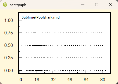
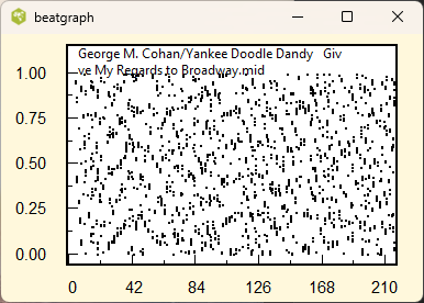
The above plots show the beatgraph for a quantized and unquantized midi files. The position of the note onset inside each beat is plotted as a function of the beat number. The music in the left plot is quantized. All the quarter, eighth, and sixteenth notes are properly aligned along a grid. The right plot was produced from an unquantized midi file. Dividing the file into equal quarter note beat intervals, the note onsets occur in random positions.
We can produce a note set histogram by computing the histogram of the note onset times modulo PPQN. (A number modulo n is the remainder when you divide the number by n.) If the midi file is quantized then, all the note onset times would occur at one of several specific times.
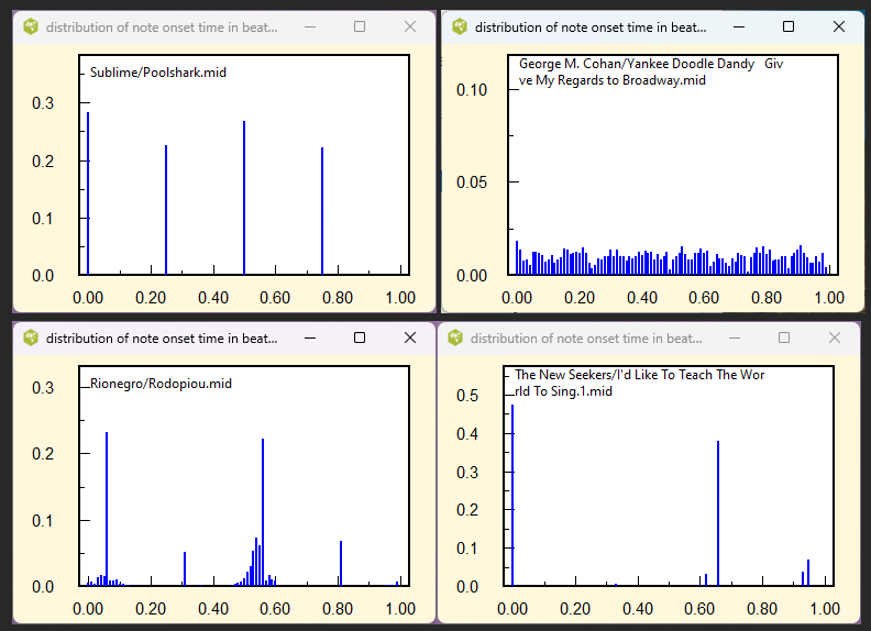
The above plots show the normalized note onset histograms (or distribution) for several midi files. The top left (Sublime/Poolshark) occurs when the music when the smallest note duration is a sixteenth note and there are no triplets. The top right is an example of unquantized note onsets. The lower left (Rionegro/Rodopiou) illustrates dithering that is applied to the quantized onsets. Performed notes do not occur at the same instant time allowing the listener to separate the distinct instruments. The lower right is an example of a distribution for music containing many triplets.
Though the note onset distribution has limited benefit in classifying the midi files, it is important when we are extracting other characteristics from the midi files. For example, if the midi file contains many triplets a resolution based on a power of two would not be ideal. The note onset distributions appear in various patterns and we are interested in knowing the frequencies of these patterns. A clustering program or a transform to a latent space would be useful.
In the above plots, the distributions are shown to a resolution of 100 time units. This leads to vectors of dimension 100. It is more convenient to work with lower dimensional vectors. A resolution of 12 time units would be sufficient to separate the effects of quarter notes, eighth, sixteenth notes and triplets. This would reduce the dimensionality of the input vectors but yet be sufficient to distinguish most of the distributions. For each of the midi files, we computed a 12-dimensional vector representing the onset distribution and stored it in a file for future analysis.
The onset time distribution shows limited variety so it was taken to be a good starting point for gaining experience with the various data analysis packages. The goal was to partition this data into smaller groups having similar properties and to determine whether these groups formed actual clusters or whether there was any sharp demarcations between the various patterns.
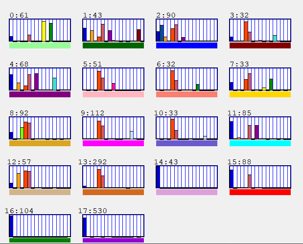
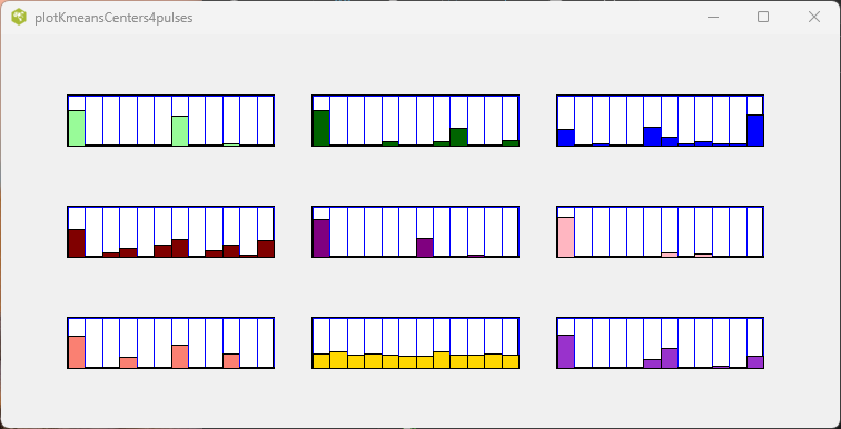
The k-means algorithm in sklearn is a well known clustering algorithm and requires one to specify the number of clusters to identify. Furthermore, the algorithm is not necessarity repeatable and returns different results each time it is run on the same data. We arbitrarily specified 9 clusters, and here are the 9 centroid vectors that it identified in one of the runs. Each of the samples, (midi files) was then assigned to one of the 9 clusters which are color coded here.
Using the same color codes we produced a scatter plot of the UMAP algorithm projection into two dimensional space. The plot below was limited to the first 3000 samples from the collection of 17,000 note onset vectors.
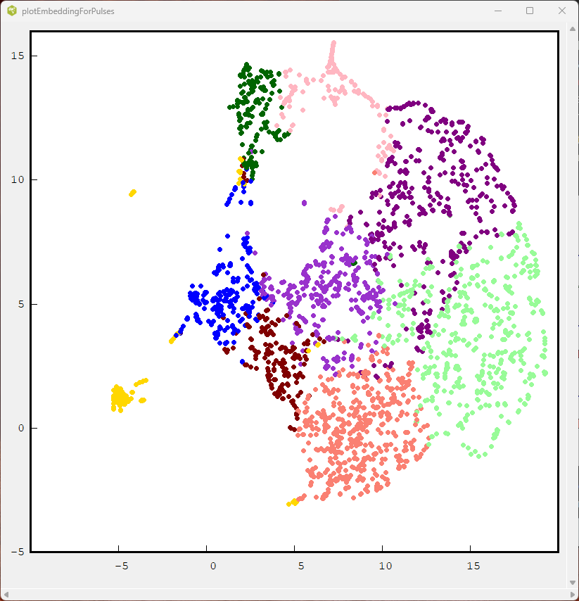
Only the set of unquantized midi files (yellow) form a distinct group. The other samples form groups that do not form distinct patterns.
It was found that neighbouring points in the UMAP mapping had similar note onset vectors.
Pitch Class Distribution
Music is composed in one the many musical scales such as D major with sharps on F and C. The music focusses on the key or tonic of the piece, so that note occurs more frequently than the other notes. Therefore the pictch class distribution shows a maximum corresponding to the key of the music.
The pitch class distribution shows how the 12 notes in the musical scale are used. Music generally restricts the usage to a set of 7 keys of the 11 possible keys determined by the key signature. Rather than ordering the notes sequential by pitch, it is preferable to order them in steps of fifths. This groups the keys belonging to a particular key signature.
Like in the previous section, we use the kmeans algorithm to partition the midi samples by their pitch class distribution and label the different clusters by different colors. The UMAP algorithm was used to visuallize the samples in a two dimensional space. Running the kmeans algorithm repeatedly with different numbers of clusters did not provide any insight in the choice to make.
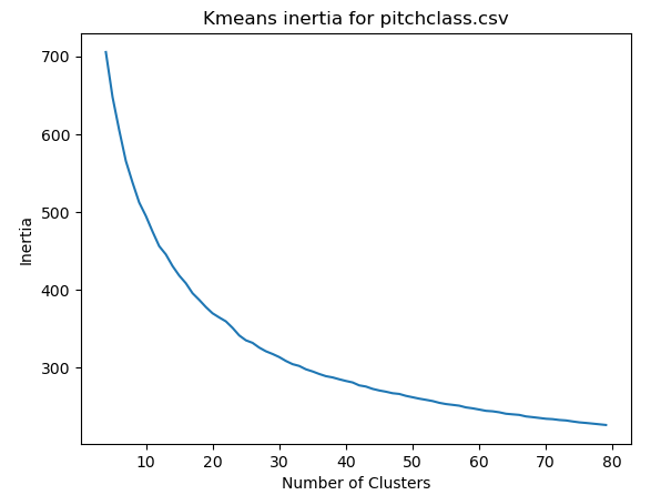
The inertia corresponds to the total root mean square error when the euclidean distance measure is used.
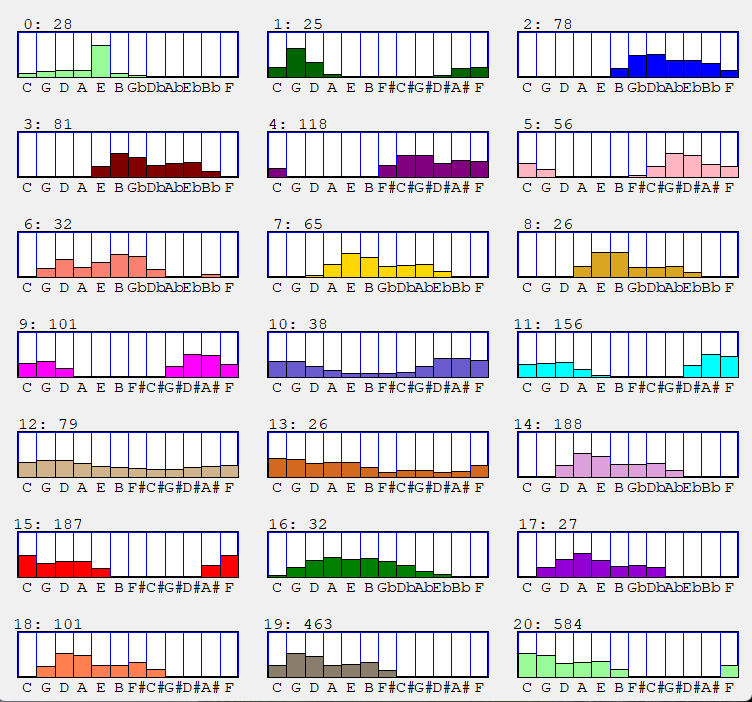
We chose to run the kmeans algorithm with 16 clusters since it would cover the number of common major and minor keys in Western music. (It is hard to find more than 16 distinctive colours. ) The centroids of the pitch class vectors for the 16 clusters are shown here. The numbers at the top left corner separated by a colon indicate the cluster number and the number of samples that were assigned to that cluster.
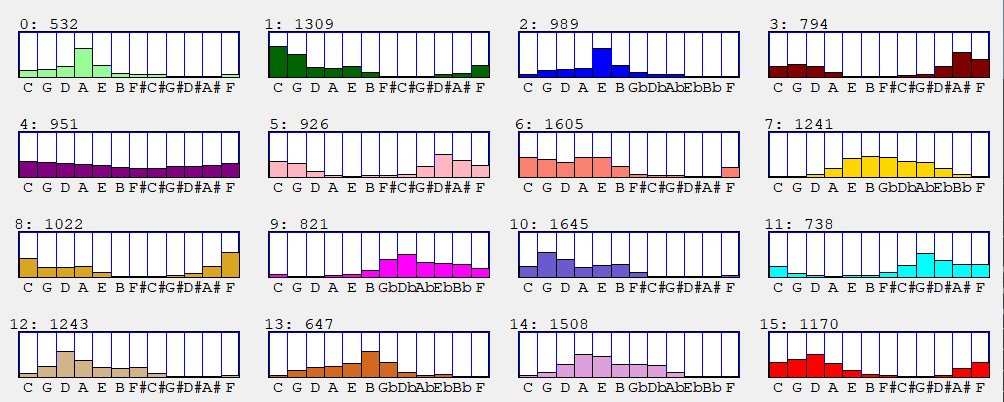
Each of the 16 cluster centroids is a vector representing the pitch class distribution of the cluster. These centroids reflect the different keys of the music. For example the top light green distribution implies the A major key. Here are the typical keys associated with the clusters.
0 A mixture 1 Cmaj 2 Emaj 3 Bbmaj 4 Mixture 5 Ebmaj 6 Amin 7 Emaj 8 Fmaj
9 F#maj 10 Gmaj 11 AbMaj 12 Dmaj 13 Bmin 14 Amaj 15 Dmin
The peak in the pitch class is not always indicative of the key center. The chordal accompaniment may dominate the distribution. The key center can shift to the dominant, subdominant, or relative minor in the piece. Furthermore, there are many samples that lie on the border of the kmean clusters. The number of samples associated should not be considered to be exact since the algorithm could converge to a different partition in another run.
Midiexplorer has the keymap function which shows how the key of the music can evolve in the midi file. The key is determined for a blocks of 20 or so beats and plotted in a color coded strip. Here is an example of the output.
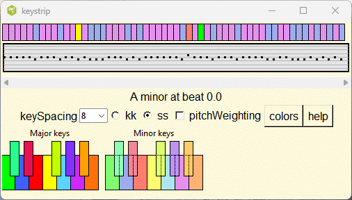
The key is fairly stable in this plot, but can jump all over the place for jazz compositions.
The HDBSCAN algorithm identified 21 clusters are shown in the plot below; however most of the sample pitch class vectors were assigned to the class representing outliers or noise and not shown here.
The choice of the input parameters to HDBSCAN was by trial and error, and the above plot is a sample result. Unfortunately, it was difficult to avoid assigning most pitch class vectors to the noise or outlier class.Though more groupings were found, some were rather similar, such as 17 and 18 or 7 and 8. Clusters 12 and 13 reflect the midi files having one or more key changes.
The Umap projection using the same color code for the kmeans centers is shown below.
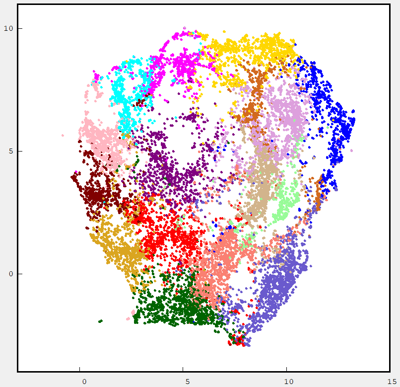
In general most of the cluster classes are well separated. The next figure shows the HDBSCAN labeled samples.
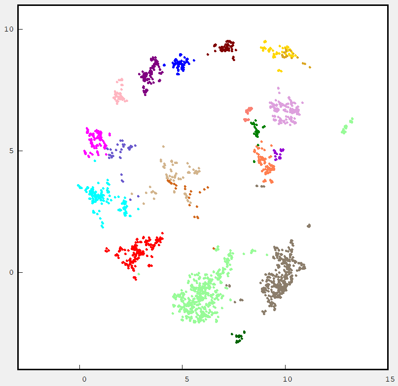
The samples that were assigned to noise or outliers are not displayed. The samples are coded in different colors compared to kmeans since HDBSCAN assigned them different cluster numbers.
With one exception, the pitch class distributions provides little information on the nature of the music in the midi file. Artists use the key which is convenient for the performers, instruments and composition.musician. The main exception is the jazz which seems to use all the 11 keys in the scale. The pitch class distribution may resemble kmeans cluster 4 or HDBSCAN clusters 12 and 13. If the music modulates to some distant key, this can cause a similar effect.
The UMAP places these flat pitch class distributions near the center. These pitch class vectors are derived from music whose keys make significant jumps. (It is not uncoomon for the music to shift up a tone near the end.) The peripheral samples tend to contain simple distributions with a sharp peak corresponding to a particular key.
We will not clutter this documents with hundreds of examples; so the reader is urged to explore this space using the umapPlot.tcl referenced above.
Program Class Distribution
The MIDI Standard defines 128 MIDI programs (musical instruments) that can be used to synthesize the notes. Some of these programs include different pianos, guitars, wind instruments, organs, and etc. The midi files use a particular subset of these programs depending on the music genre and style. For example, blue grass music typically has a banjo and a fiddle. Heavy metal has either a distortion guitar or overdriven guitar or both. For this reason, we may expect to find clusters of midi files that have similar midi program subsets.
It is rather difficult dealing with 128 dimensional vector indicating the use of all the available programs for each of the midi files. To reduce the size of the vector, it was convenient to partition these programs into 16 groups . The groupings are defined in MidiExplorer (sourceforge.io) which refer to as program classes. For each midi file, the amount of activity in each of the program classes was computed and stored in the program class vector. Here is a table of the different program classes.
| piano keyboard | xylophone category | acoustic guitar category |
| organ class | electric guitar set | electric bass set |
| solo strings (eg. violin) | string ensembles | choir |
| brass | drum class | woodwind |
| flute category | lead class | pad class |
| FX class | Banjo class | electronic synthesizer |
There are many issues with dealing with the program class vectors. First there is the question on how to compute this vector. Not all the midi instruments are playing at the same time. Some instruments may only play a couple of notes. The program class vector should give larger weight to the classes which are active over a longer period of time. Therefore if a flute is playing a note continuously over the entire midi file, it is given a weight of 1.0. If the flute plays for less than half the time, then its weight will be less than 0.5. If the flute is playing in one channel and the recorder (another instrument in the flute category) in another mdi channel then their contributions should add up. Thus it is possible to have a value greater than 1.0 for the flute category. The next question is how to normalize the program class vector. We can normalize it like a probability distribution, so that the sum of all the vector components add up to 1.0. Alternatively, we can normalize it so that the euclidean length of the program class vector is always 1.0. Finally, how do we compare two program class vectors. There are many distance metrics such as euclidean, manhattan, chebyshev, and many more which all yield different answers. The metric that we use effects the behaviour of clustering and dimensionality reduction algorithms.
The Lakh clean dataset contains many different interpretations of same music. They are indicated by midi file names with the same name but a different numeric extension. The midi instruments that are used are often different in the interpretations. This introduces another level of variability in the program class vectors. If the variability is too large, none of the analysis algorithms will perform well. In fact this is the actual situation.
It was rather difficult choosing the right input parameters for these analysis algorithms. In addition there is a choice of whether to scale all the vector components to the same range. To compound the situation, all of these algorithms are stochastic in nature and converge to different solutions each time they are run. Here are some of the results.
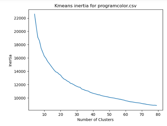
The inertia error for the kmeans algorithm decreased slowly with the number of clusters.
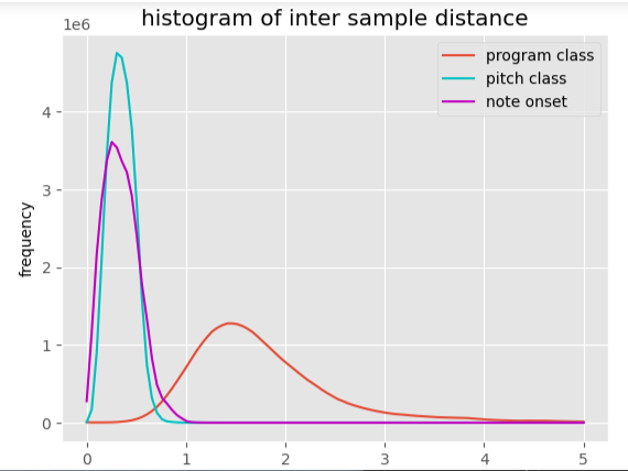
The intersample distances were much higher for the program color vectors in comparison with the other vector collections.
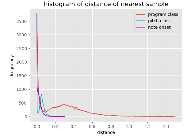
The histogram of the distance to the nearest neighbouring sample was also broader for the program color vectors.
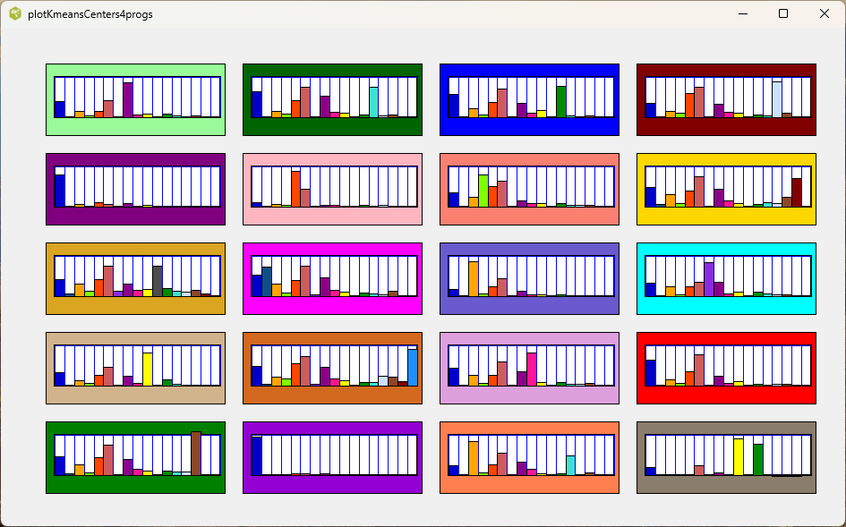
The kmeans cluster centers were not easy to interpret and did not relate well to the midi file styles.
Finally the UMAP output did not localize some of the clusters very well.
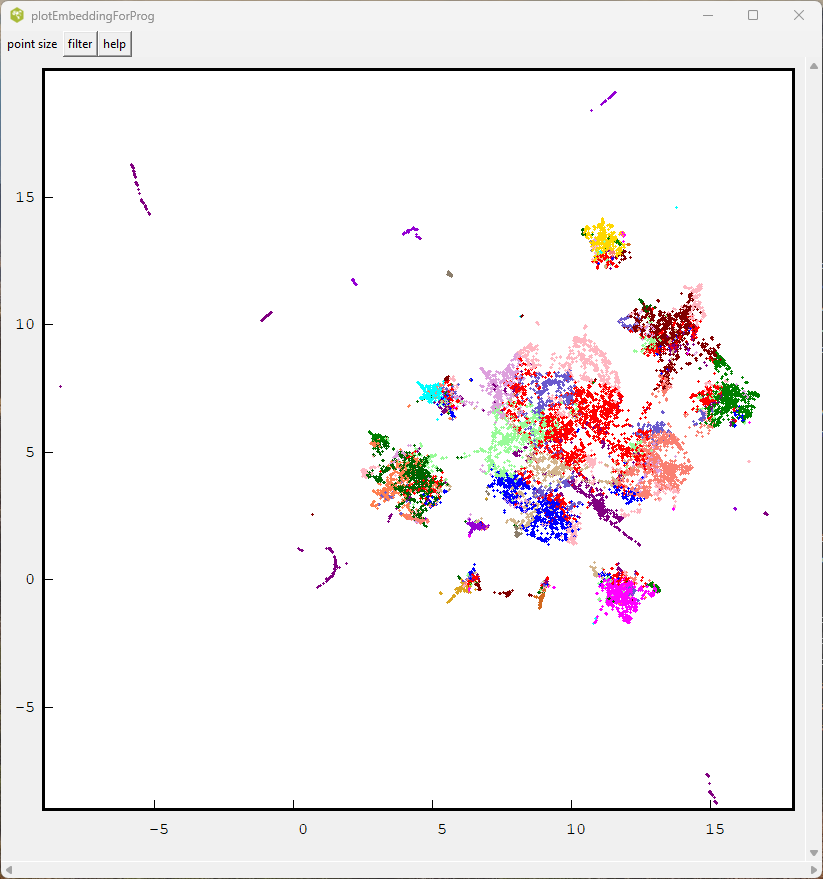
The HDBSCAN algorithm tended to classify more than 90 percent of the samples as noise or outliers; however the few clusters (peaks) that it did find were less complex.